Grounded persistent path homology: a stable, topological descriptor for weighted digraphs
Posted to site: 25/10/22
Weighted digraphs are used to model a variety of natural systems and can exhibit interesting structure across a range of scales. In order to understand and compare these systems, we require stable, interpretable, multiscale descriptors. To this end, we propose grounded persistent path homology (GRPPH) - a new, functorial, topological descriptor that describes the structure of an edge-weighted digraph via a persistence barcode. Joint work with Heather A. Harrington and Ulrike Tillmann.
Project Summary
Persistent path homology (PPH) combines path homology (a homology theory for digraphs) and persistent homology (a tool for developing multiscale statistics). The input to PPH is a directed network and the output is a barcode; the pipeline is stable.
But what if I have a weighted digraph and I care about its underlying topology? As a first attempt, let’s compute the shortest-path quasimetric (a directed network) and then measure PPH.
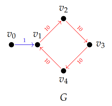
This is a natural pipeline, but it has a problem! Consider this example; all edges in \(G_1\) have weight \(1\) and all edges in \(G_2\) have weight \(0.5\). The smaller holes in \(G_1\) are filled in as soon as they are born (by long squares at \(t=1\)). After subdividing, we recover the small features and birth times reduce.
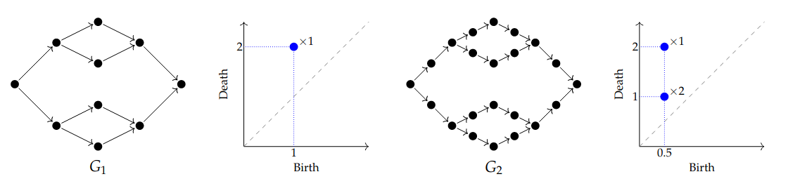
This raises an issue for interpretation: the number of “holes” changes upon subdivision. The underlying graph already had three “holes” but our pipeline does not respect them. Moreover, representatives for the features do not naturally live in G.
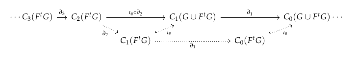
To fix this issue, we introduce grounded persistent path homology (GrPPH). We alter the path homology chain complex so that all edges in G are born at time 0, but generators in degree 2 appear at the same time.
The number of features in the resulting barcode is equal to the circuit rank of the underlying graph. Moreover, we show there is a choice of undirected circuits, which form a basis for the cycle space and a persistence basis for GrPPH. The geometric nature of these representatives make them ideal for interpretation.
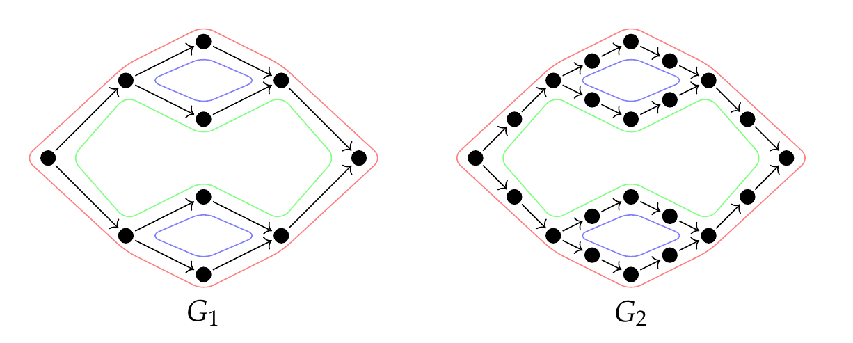
Back to our working example, \(G_1\) and \(G_2\) end up with the same barcode: \(\{\!\{[0, 1), [0, 1), [0, 2)\}\!\}\). Below, the small features are represented in blue and the larger feature in green (or red).
GrPPH is a functor from a category of weighted digraphs, where morphisms are maps of the underlying digraphs and contractions of the shortest-path quasimetric. This allows us to compare the GrPPH of digraphs related by such morphisms.
We find stability to weight perturbation and edge subdivision, as well as some edge collapses and edge deletions. As a corollary, GrPPH (and indeed PPH) converges under iterated subdivision.
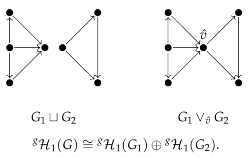
We also show that GrPPH decomposes as a direct sum when G decomposes as a disjoint union or wedge sum. This is a boon for interpretation and computation: if an edge or a vertex belongs to no simple circuit, we can delete it without affecting GrPPH.
For completeness, we apply the same methodology to the directed flag complex. We find that weaker functoriality leads to an instability; deleting the blue edge below changes the barcode from \(\{\!\{[0, 21)\}\!\}\) to \(\{\!\{[0, 30)\}\!\}\).
When using GrPPH, the two persistent vector spaces are isomorphic.
Software
If you would like to use GrPPH to study your data, install our python library with:
pip install grpphati
Current features include:
- Grounded persistent path homology
- Grounded persistent directed flag complex homology
- Support for grounded pipelines with custom homology theories and filtrations
- Cycle representatives
- Parallelisation over wedge and disjoint union decompositions
- Support for multiple PH backends, including Eirene and PHAT
Documentation is still a work in progress but informative examples are avilable on the GitHub repo.
If you need a more performant library, check out grpphati-rs which boosts grpphati with Rust-accelerated boundary matrix construction.
If you would like to get started right away, without installing anything, then you can clone and start working on this Google Colab notebook.
Computational Examples
Consider the following toy vascular networks which are modelled as follows:
- Each edge is assigned a length \(L\) and a cross-sectional area \(A\).
- Each node is given a net current (most are 0 except inlets and outlets).
- the network is modelled as an electrical resistance network with edge resistance \(R = L/A \).
- Kirchoff’s laws yield a system of linear equations which we solve for the current \(I\) in each edge.
- Each current is converted to a time via \(T = (L * A) / I \).
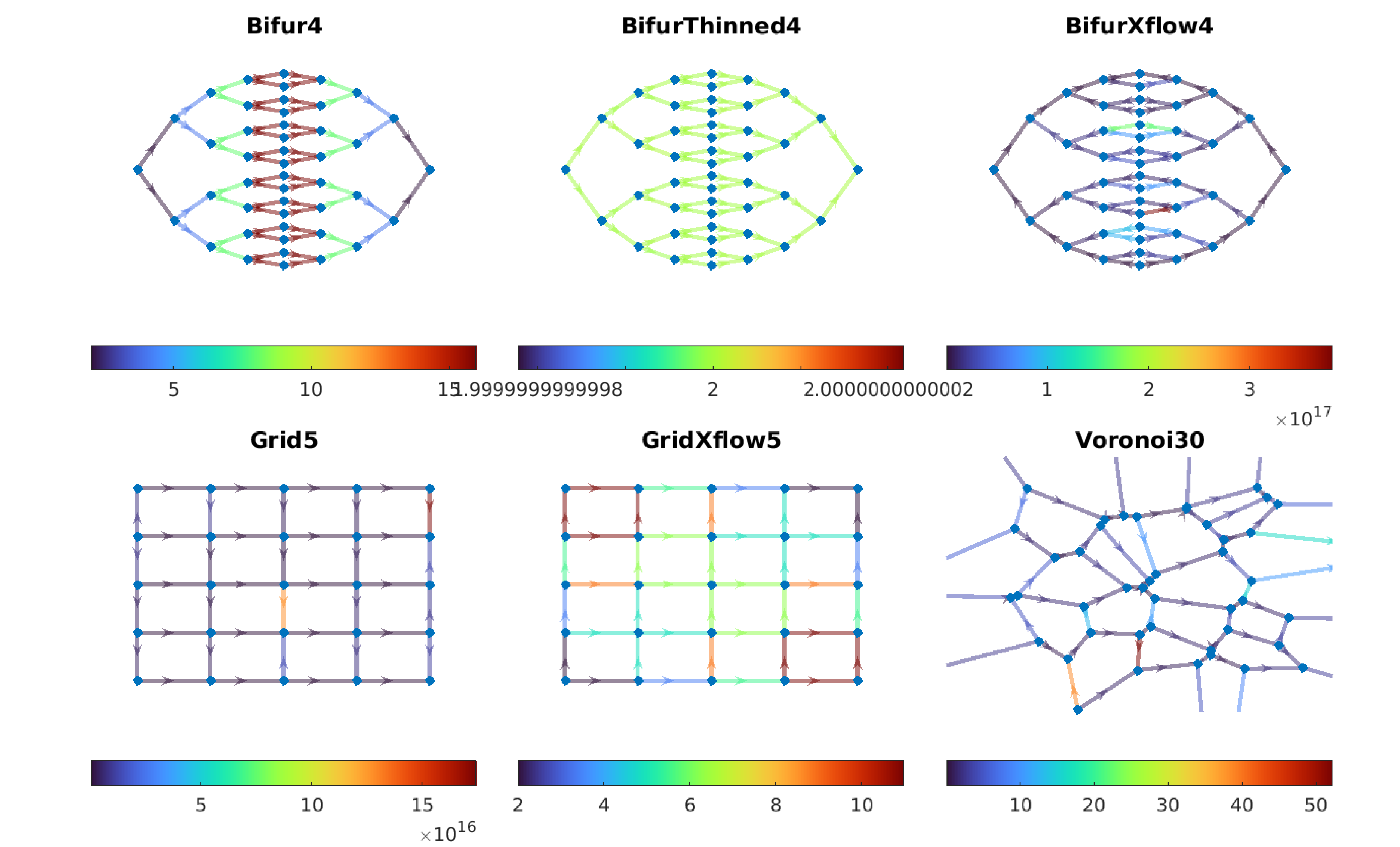
Note the following difference between the networks:
- BifurThinned4 has thinner edges towards the middle and hence a constant edge weight.
- BifurXflow4 has one inlet at the bottom and one outlet at the top. Only the outer edges received flow.
- Grid5 has flow left to right and the vertical edges are ununes.
- GridXflow5 is diagonally loaded and hence all edges are used.
We then measure GrPdFlH of each of these networks and compute the Betti curves.
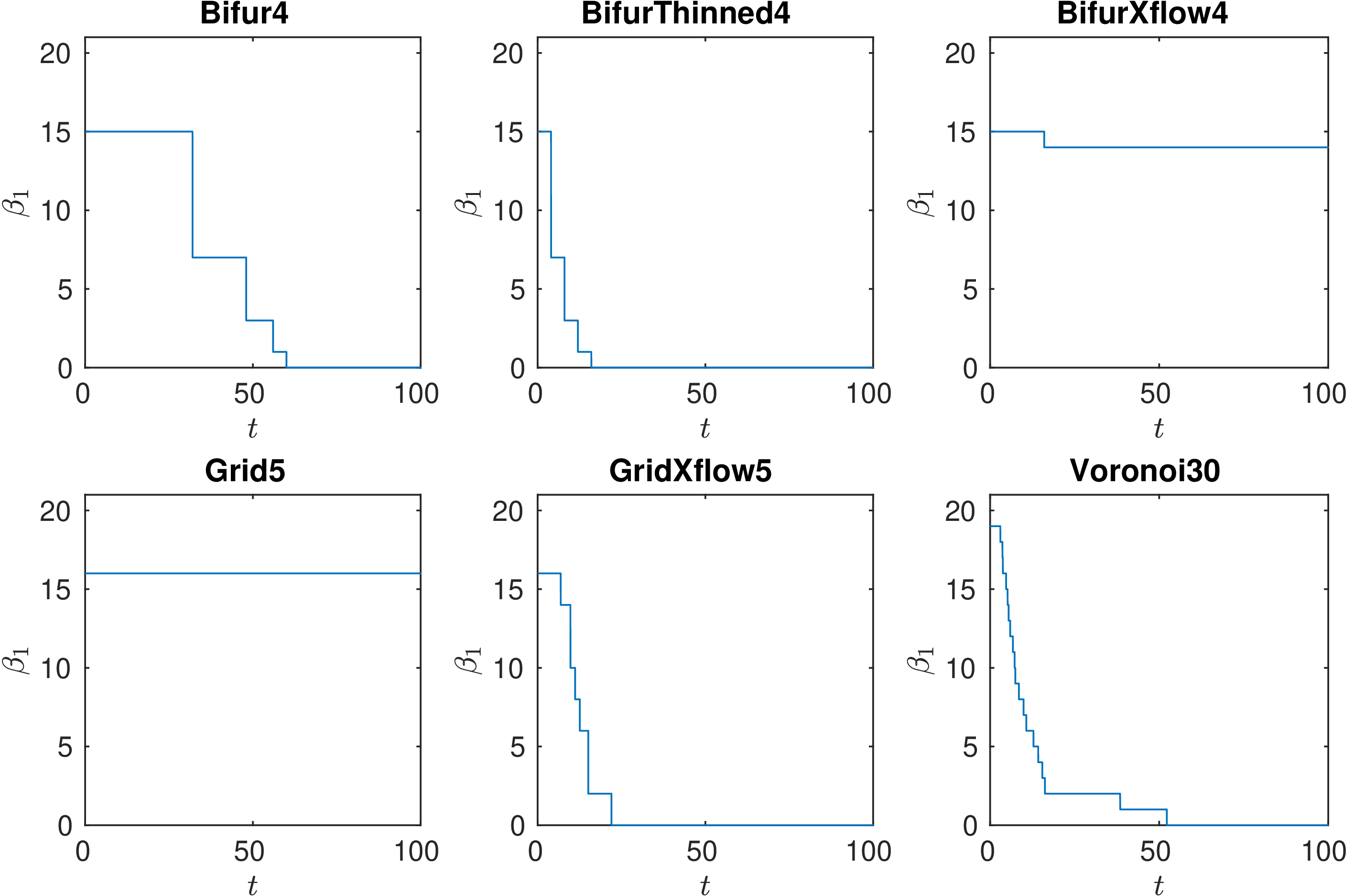
Some observations:
- Bifur4 has no large holes in the flow and hence all features die quickly.
- Thinning edges towards centre of bifurcation network increases flow velocity so features die quicker in BifurThinned4.
- Inducing cross flow means edges in the centre get 0 flow. Hence all features are long-lived, apart from outer loop in BifurXflow4.
- In Grid5, the flow doesn’t use vertical edges so all features are long-lived.
- In GridXflow5 the flow uses all edges so the features die more quickly.
- Voronoi30 has similar descriptor to the bifurcation network but has a few long-lived features.
To assess the stability of each of these networks we now subject the networks to two random perturbations
- Random independent each removal, with probability \(p\).
- Random edge shuffling, with \(N\) attempted shuffles.
To make the stability differences more comparable, we normalise each Betti curve by its maximum value at \(t=0\).
Note that the bifurcation networks are more unstable to these pertubations, when compared to the Voronoi network, despite the similar initial descriptor.