Exploring the Mandelbrot Set

Posted to site: 02/11/18

GitHub

The Mandelbrot set has be­come an am­bas­sador for the beauty of math­e­mat­ics. Its hyp­notic, com­plex struc­ture has as­tounded math­e­mati­cians and non-math­e­mati­cians alike, and has been a sub­ject of math­e­mat­i­cal re­search for decades. Interested in the struc­ture and be­hav­iour of the Mandelbrot set, I used Python to an­i­mate zooms into this cap­ti­vat­ing frac­tal. The lim­i­ta­tions of in­ter­preted lan­guages like Python soon be­came clear so I turned to multi-threaded tech­niques and C++ to speed things up.

Formal Definition

To for­mally de­fine the Mandelbrot set, for every \(c\in\mathbb{C}\) we de­fine the func­tion \( f_c: \mathbb{C}\to\mathbb{C},;z\mapsto z^2 + c \) and sub­se­quently the se­quence \( \left( z_{c,n} \right)_{n=0}^\infty \) by \(z_{c,0}=0\) and \(z_{c,n+1}=f(z_{c,n})\). Now we can de­fine the Manelbrot set to be the set of points \(c\in\mathbb{C}\) such that \( \left( z_{c,n} \right)_{n=0}^\infty \) is bounded.

We would like to draw a pic­ture of the Mandebrot set, but de­ter­min­ing whether a se­quence is bounded would re­quire com­put­ing the en­tire in­fi­nite se­quence which is quite a long job. In or­der to com­pute whether a given point of the com­plex plane lies within the Mandelbrot set, we re­quire a sim­pler cri­te­rion. Thus, we in­tro­duce an es­cape ra­dius \(r>0\) which we choose with the prop­erty that if \(|z_{c,n}|>r\) for some \(n\in\mathbb{N}\) then we may con­clude \(c\not\in M\). It can be shown quite sim­ply that 2 is an es­cape ra­dius.

We now have a very sim­ple al­go­rithm for de­ter­min­ing whether or not a point lies in the Mandelbrot set. We com­pute the se­quence \( \left( z_{c,n} \right) \) and, if it any point we see that \(|z_{c,n}|>2\), then we can con­clude that \(c\not\in M\). Unfortunately, we can’t keep do­ing this for­ever so we must de­cide be­fore hand on a max­i­mum num­ber of points in the se­quence we are will­ing to com­pute, be­fore we give up and guess that \(c\) be­longs to the Mandelbrot set. Of course, the more it­er­a­tions we com­pute, the more ac­cu­rate our draw­ing of the man­del­brot set be­comes.

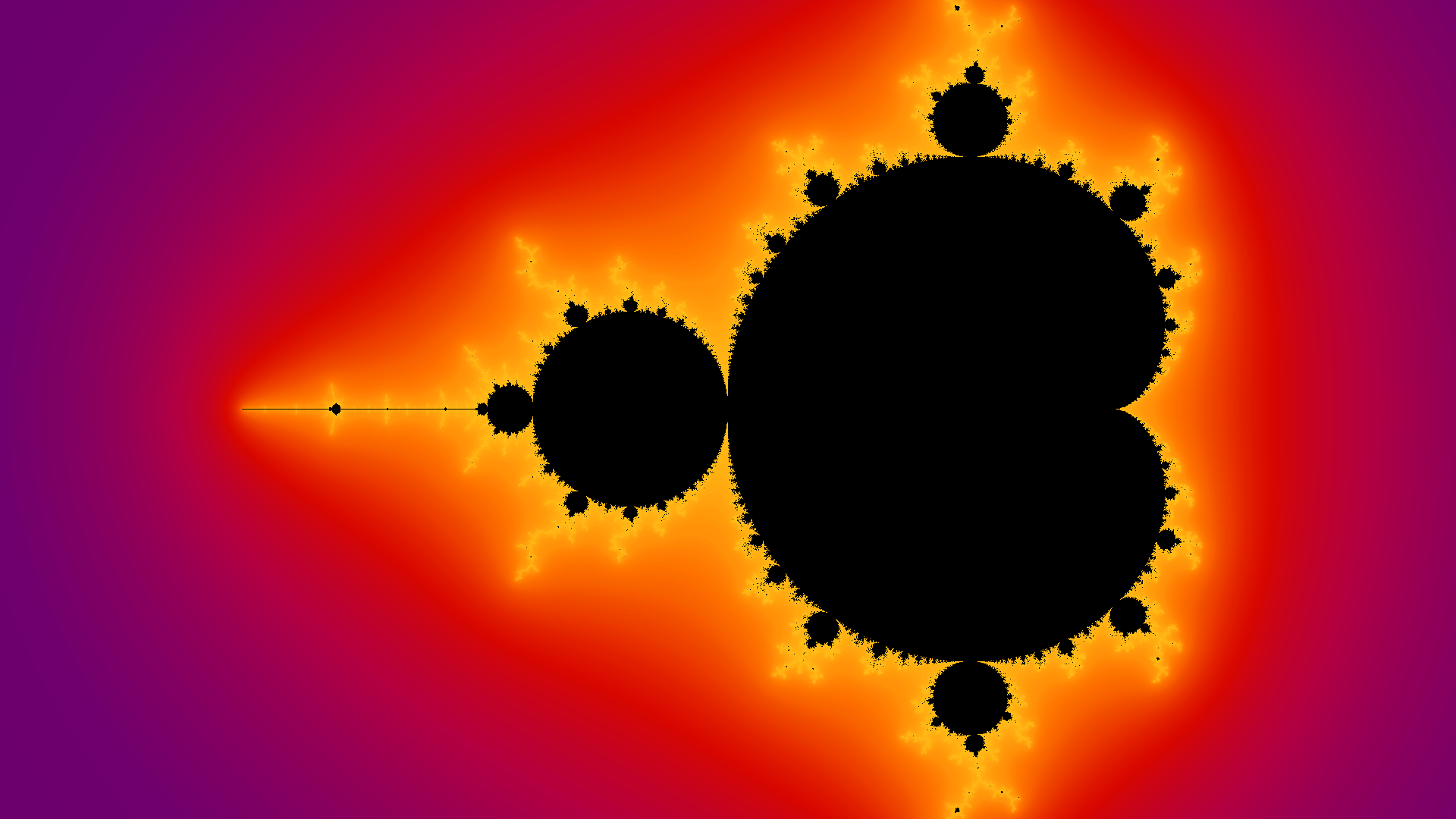
But we can do bet­ter. For all for the points we know lie out­side of the Mandelbrot set, we also know how long it took for the se­quence to es­cape. If a point es­capes very quickly then, in some sense, it is very far away from the set. Therefore, based on how many it­er­a­tions it took for the se­quence to es­cape, we can colour in each point in \(\mathbb{C}\), based on how close it is to be­ing in the Mandelbrot set.

Colouring

There are a num­ber of meth­ods for colour­ing in the Mandelbrot set. All of the meth­ods start with a pal­lete of colours. One ap­proach would be to map 0 it­er­a­tions to the first colour, the max­i­mum num­ber of it­er­a­tions to the last colour and then lin­early in­ter­po­late all colours in­be­tween. This pre­sents a prob­lem as we zoom into the set, be­cause points very close to each other will take roughly the same num­ber of it­er­a­tions to es­cape and thus will be coloured very sim­i­larly pro­duc­ing a rather bor­ing, mo­not­one im­age. One fix to this would be to pick a rel­a­tively small palette and keep loop­ing around the palette. For ex­am­ple, if we take a pal­lete of 100 colours then we would colour a point the same if it took 0 it­er­a­tions or 100 it­er­a­tions.

This pro­duces a colour­ful im­age but we have now lost the prop­erty that one side of our palette is ‘closer’ to the Mandelbrot set than the other. The so­lu­tion to this is a method known as his­togram colour­ing. We start by mak­ing a his­togram where we count how many pix­els took each num­ber of it­er­a­tions to es­cape. We then use this to map each it­er­a­tion num­ber to a colour in the palette. This en­sures that the first and last colours are used so the pic­tures will use the full range of colours ava­iable in the palette so we get pic­tures with much bet­ter con­trast.

---

---

---

---

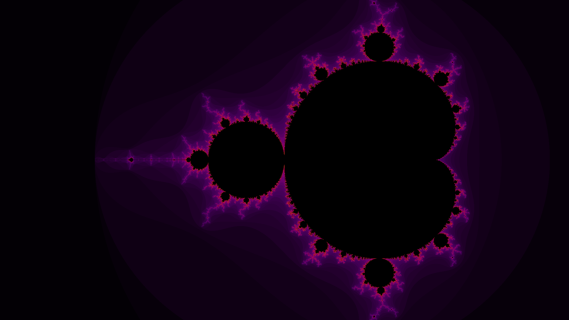
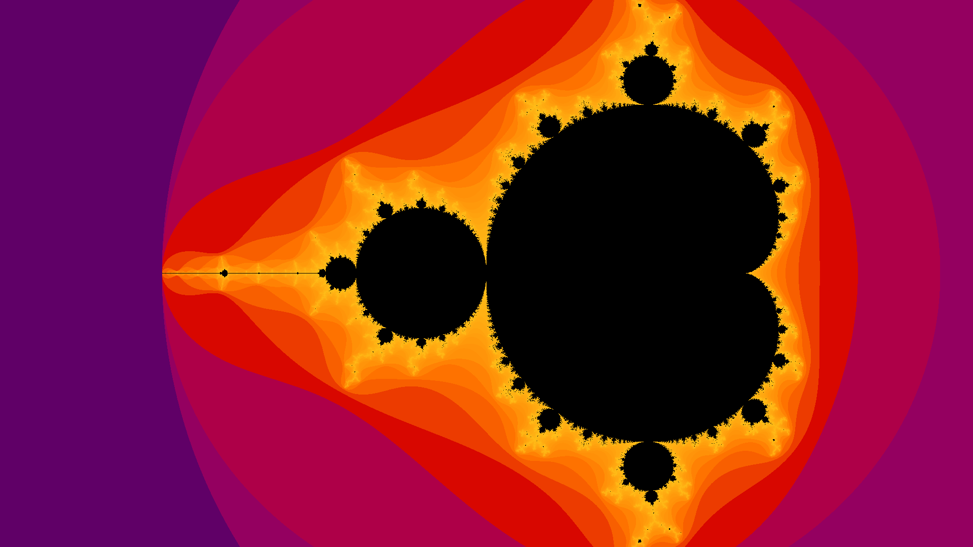
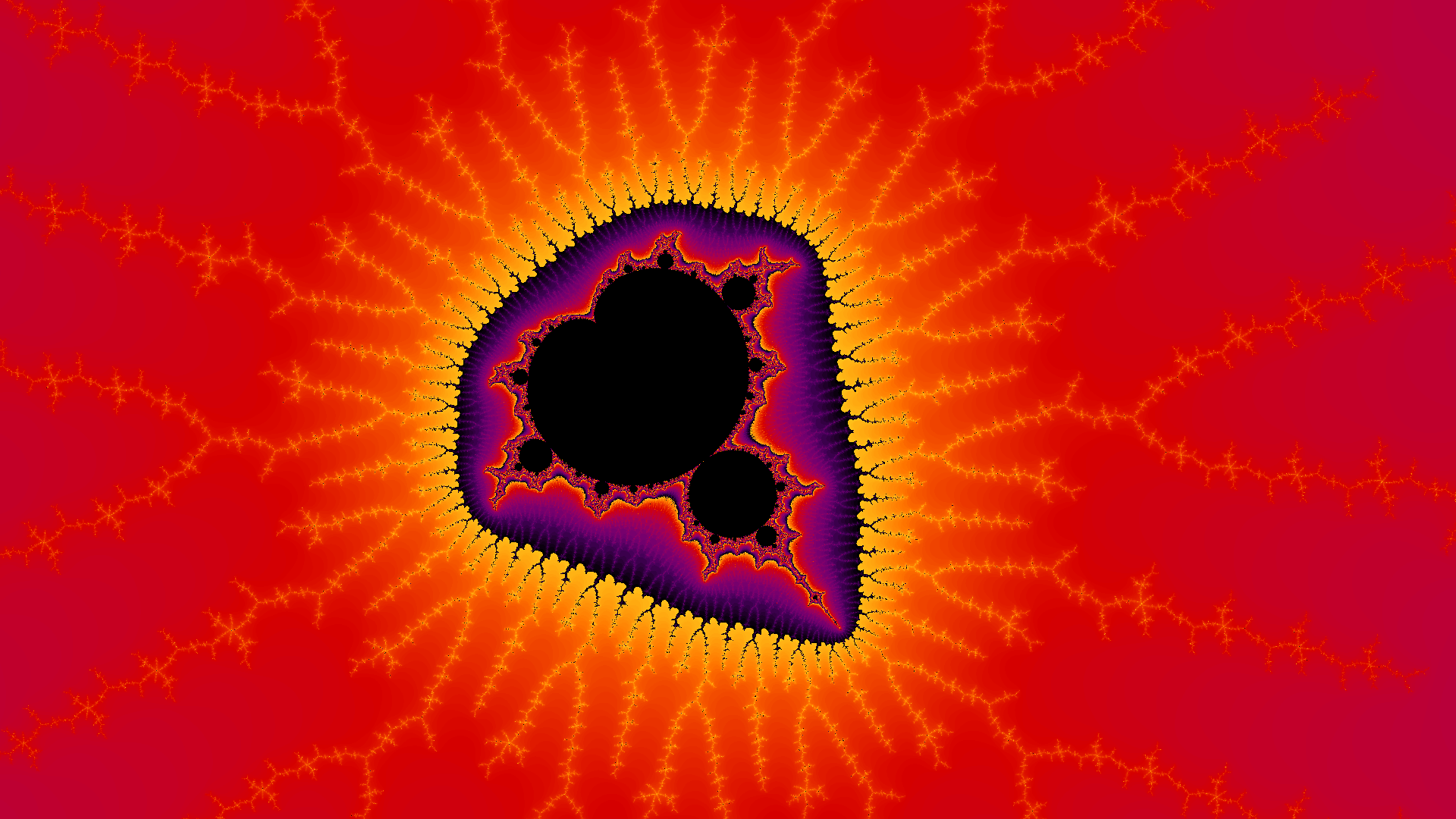
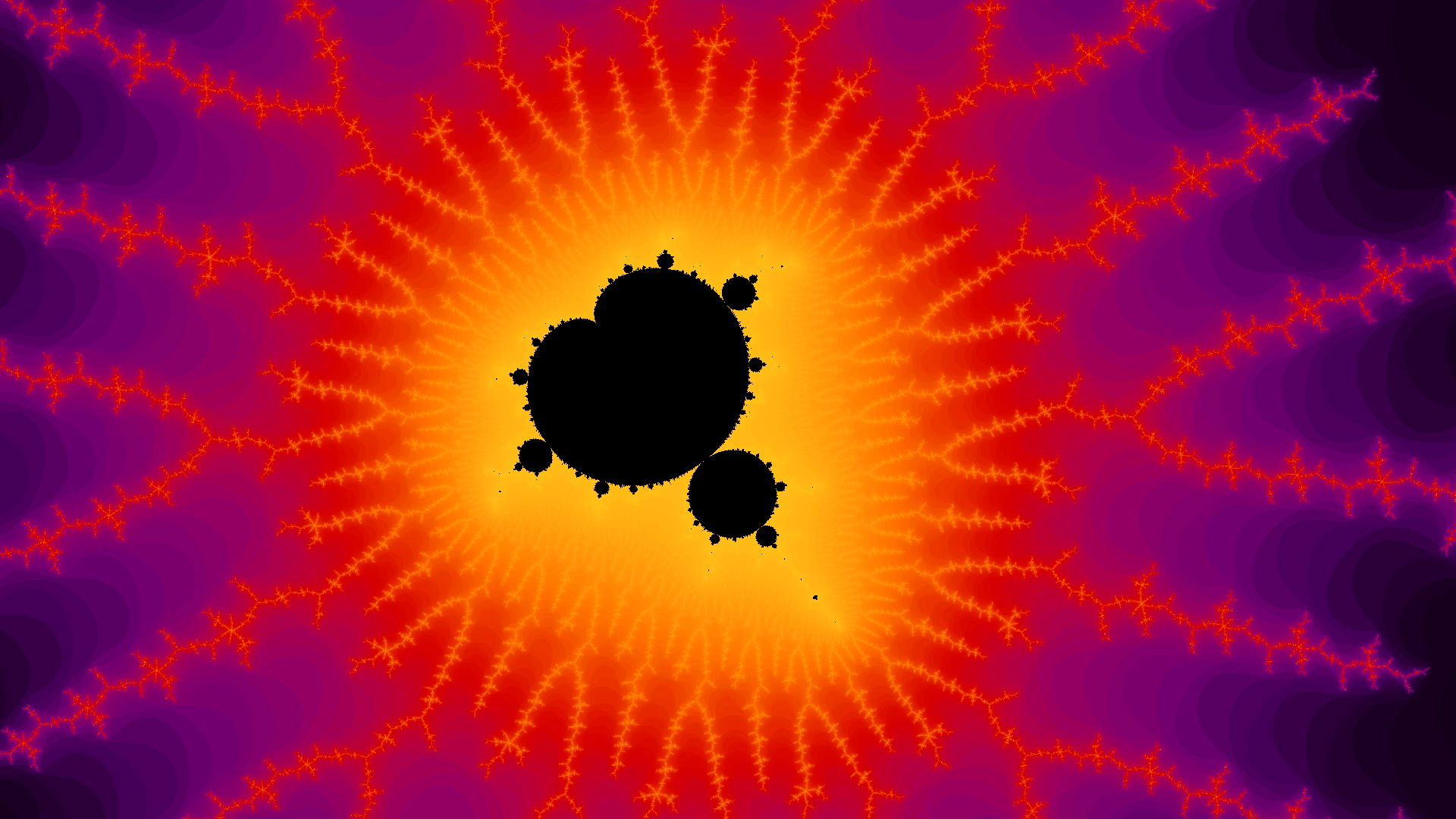
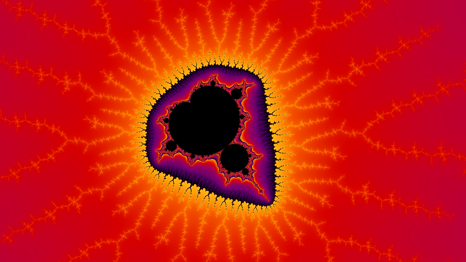
This is clearly a much bet­ter way to colour our Mandelbrot set if we wish to re­tain de­tail as we zoom into the set as we can guar­an­tee that we will use the full range of colours in our palette. However, from an artis­tic view­point, these im­ages are still lack­ing some­what. Since we are colour­ing based on a dis­crete prop­erty (the num­ber of it­er­a­tions to es­cape), we end up with dis­crete jumps be­tween colours in our palette, cre­at­ing clear bands of colour. We would pre­fer to see a con­tin­u­ous change from one colour to the next so we need a prop­erty sim­i­lar to it­er­a­tion num­ber which can take on any real value, not dis­crete in­te­gers.

The prop­erty which solves this prob­lem is known as the nor­malised it­er­a­tion count. For an ex­pla­na­tion of this colour­ing al­go­rithm, please see this ex­cel­lent post by Linas Vepstas.

---

---

---

---

Multithreading with thread pools in C++

The curse of the Mandelbrot set is that com­put­ing the colour of one pixel tells you al­most noth­ing of use about the ad­ja­cent pix­els. Indeed it is this prop­erty that gives the set its in­trigu­ing frac­tal na­ture. However, this does leave the prob­lem of com­put­ing pic­tures of the Mandelbrot set es­pe­cially sus­cep­ti­ble to par­al­leli­sa­tion; em­barass­ingly so. Since all of the pix­els can be com­puted in­de­pen­delty and in any or­der, we can levarage the power of a multi-core proces­sor or even a clus­ter of proces­sors, with­out wor­ry­ing about syn­chro­ni­sa­tion prob­lems.

In this pro­ject, I used a sim­ple sin­gle-header C++ li­brary which im­ple­ments the thread pool de­sign pat­tern. This pat­tern con­sists of a num­ber of threads or “workers” and a con­tainer of jobs. As jobs are pushed to the con­tainer, idle work­ers take jobs out of the con­tainer and com­plete them. This pre­vents the re­peated cre­ation and dele­tion of work­ers through­out the com­pu­ta­tion, re­duc­ing the com­put­ing re­sources spent on par­al­leli­sa­tion and in­creas­ing ef­fi­cieny. Moreover, this ap­proach is eas­ily scal­able to com­put­ers with a larger num­ber of avi­l­able of proces­sors as this sim­ply re­quires cre­at­ing more work­ers and adding them to the pool.

Working Code

In the GitHub repo for this pro­ject, I have in­cluded a Python file which im­ple­ments the Hisogram colour­ing al­go­rithm in a se­r­ial fash­ion. This is quite a slow script due to the nat­ural lim­i­ta­tions of Python and lack of par­al­leli­sa­tion.

The main con­tent lies in the C++ Mandelbrot class. This is a flex­i­ble class that al­lows you to eas­ily draw pic­tures of the Mandelbrot set to a GIF, us­ing any one of the colour­ing al­go­rithms de­scribed above and any num­ber of threads. For an ex­am­ple of how to use this class, please con­sult the README on the GitHub repo. Below I have pro­vided ex­am­ples of zooms into the Mandelbrot set us­ing the smooth his­togram colour­ing al­go­rithm.

---

---

Next Steps

This C++ class could be used to im­ple­ment an in­ter­ac­tive ex­plorer (sim­i­lar to this on­line ex­plorer) which would be able to lever­age the power of par­al­lel com­put­ing to ex­plore the struc­ture of the Mandelbrot set. Moreover, this ex­plorer could first ren­der the im­ages in a lower res­o­lu­tion, al­low­ing the user to quickly plot a path. The pro­gram could then trace back along this path at a higher res­o­lu­tion to pro­duce an in­ter­est­ing zoom.

When an­i­mat­ing zooms into the Mandelbrot set, choos­ing a cen­tre point is rather cru­cial to ob­tain­ing a sat­is­fac­tory re­sult. If poorly cho­sen, the an­i­ma­tion will of­ten re­sult in an in­def­i­nite zoom into black­ness. For ex­am­ple, zoom­ing di­rectly into the cen­tre of the Mandelbrot set would be some­what dull. To fix this, we could im­ple­ment a sys­tem which analy­ses the pre­vi­ous frame and sub­se­quently makes small ad­just­ments to the cen­tre point in or­der to en­sure that we keep zoom­ing into some­thing of in­ter­est. The sys­tem could then be left com­put­ing with less su­per­vi­sion, zoom­ing into the Mandelbrot set un­til it ran into er­rors due to float­ing point pre­ci­sion. This would also re­quire suit­ably in­creas­ing the max­i­mum num­ber of it­er­a­tions per pixel as we zoom in, so as to en­sure that we re­tain some level of de­tail.

To fur­ther in­crease the com­pu­ta­tion speed of this pro­gram, one could use the worker pool de­sign pat­tern to dis­trib­ute work across a clus­ter of com­put­ers such as Raspberry Pis. Alternatively, or even ad­di­tion­ally, the pro­gram could be rewrit­ten to lever­age GPU ac­cel­er­a­tion, al­though such a pro­gram would in­her­ently be more tai­lored to a spe­cific com­puter. Another way to speed up com­pu­ta­tion of the Mandelbrot set is through perbu­ta­tion the­ory. Ultra Fractal now sup­ports the ‘perbutation cal­cu­la­tion al­go­rithm’ which al­lows you to ap­prox­i­mately cal­cu­late the it­er­a­tion for points close to a point that has al­ready been cal­cu­lated. This al­go­rithm was first dis­cov­ered and im­ple­mented by K.I. Martin and the math­e­mat­ics and al­go­rithm are de­tailed on the SuperFractalThing web­site.

These tech­niques of par­al­leli­sa­tion could be ap­plied to sim­i­lar frac­tal struc­tures and dy­nam­i­cal sys­tems in the com­plex plane such as Julia sets.

Update (circular colour­ing)

I have im­ple­mented some more colour­ing al­go­rithms into the C++ class. These are all cir­cu­lar colour­ing al­go­rithms which loop the pro­vided colour palette around the ori­gin as shown in the pic­ture be­low. The colour is cho­sen based on the hue and sat­u­ra­tion from the colour palette and then lu­mi­nance is cho­sen based on it­er­a­tion count so that we can see the Mandelbrot struc­ture. I have im­ple­mented this with a nor­mal colour­ing al­go­rithm as first de­scribed, as well as a his­togram ver­sion and smooth ver­sion us­ing sim­i­lar tech­niques to be­fore.

---

---

In the above pic­ture I used a palette which loops around hue from 0 to 360 de­grees with sat­u­ra­tion fixed at 50%. Obviously the colour­ing ef­fect is cen­tred at the ori­gin so as you zoom in the colour­ing will be­come mono­chro­matic, but the shad­ing will still re­veal the struc­ture of the Mandelbrot set.

Update (MPI)

I have re­cently built a small su­per-com­puter con­sist­ing of four Raspberry Pi 4s. As such, I have started the work of trans­lat­ing this code to MPI so that the work­load can be dis­trib­uted across a list of com­put­ers on the net­work via SSH. While this is still in its in­fancy, the code is avail­able here. At the mo­ment the code dis­trib­utes the work­load a row at a time> How­ever, in prin­ci­ple, we could write the code in se­r­ial to com­pute an en­tire frame, based on com­mand-line pa­ra­me­ters, and then dis­trib­ute the work via GNU Parallel.

Useful Resources

• Renormalising the Mandelbrot Set - Read more about smooth colour­ing of the Mandelbrot set
• Coloring Dynamical Systems in the Complex Plane - Read more about colour­ing al­go­rithms for dy­nam­i­cal sys­tems
• Thread Pools on Wikipedia - A ba­sic back­ground on the thread pool de­sign pat­tern
• Interactive Web Mandelbrot Explorer - Particularly use­ful for find­ing in­ter­st­ing points to zoom into
• Ultra Fractal - Excellent piece of soft­ware, used for gen­er­at­ing im­ages of a va­ri­ety of frac­tals in­clud­ing the Mandelbrot set
• SuperFractalThing - First im­ple­men­ta­tion of the perbu­ta­tion cal­cu­la­tion al­go­rithm